REDCap is an electronic data capture software that is widely used in the academic research community. The REDCapR package streamlines calls to the REDCap API from an R environment. One of REDCapR’s main uses is to import records from a REDCap project. This works well for simple projects, however becomes ugly when complex databases that include longitudinal structure and/or repeating instruments are involved.
The REDCapTidieR package aims to make the life of analysts who deal with complex REDCap databases easier. It builds upon REDCapR to make its output tidier. Instead of one large data frame that contains all the data from your project, you get to work with a set of tidy tibbles, one for each REDCap instrument.
Case Study: The Superhero Database
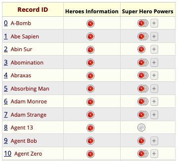
Let’s look at a REDCap project that has information about some 734 superheroes, derived from the Superhero Database.
Here is a screenshot of the REDCap Record Status Dashboard of this database. It has two instruments, Heroes Information which captures “demographic” data about each individual superhero such as their name, gender, and alignment (good or evil), and Super Hero Powers which captures each one of the superpowers that a specific superhero possesses.
Importing data from REDCap
To import data from REDCap, use the
read_redcap() function. read_redcap() requires
a REDCap database URI and a REDCap
API token. You need to have API access to the REDCap database to
use REDCapTidieR. REDCapTidieR does not work with files exported from
REDCap. We use it here to import data from the Superheroes
database. You can see that it returns a tibble named superheroes.
We use rmarkdown::paged_table() so you can explore this
tibble.
library(REDCapTidieR)
superheroes <- read_redcap(redcap_uri, token)

superheroes |>
  rmarkdown::paged_table()
You can see that the tibble that read_redcap() returned
has only two rows. This may be
surprising because you might expect more rows from a database with 734
superheroes. read_redcap() returns data in a special object
that we call the supertibble. The
supertibble contains, among other things, tibbles with the data and
metadata derived from each instrument. We call these the data tibbles and
metadata
tibbles.
Each row of the supertibble corresponds to one REDCap
instrument. The redcap_form_name and
redcap_form_label columns identify which instrument the
row relates to. The redcap_data column contains the data
tibbles. The redcap_metadata column contains the metadata
tibbles. Additional columns contain useful information about the data
tibble, such as row and column counts, size in memory, and the
percentage of missing values in the data.
Exploring the contents of the supertibble
We designed the supertibble so you can explore it with the RStudio Data Viewer. You can click on the table icon in the Environment tab to view of the supertibble in the data viewer. At a glance you see an overview of the instruments in the REDCap project.
superheroes
supertibbleYou can drill down into individual tables in the
redcap_data and redcap_metadata columns. Note
that in the heroes_information data tibble, each row
represents a superhero, identified by their record_id.
heroes_information data tibbleIn the super_hero_powers data tibble, each row
represents a superpower of a specific hero. Each row is identified by
the combination of record_id and
redcap_form_instance. This difference in granularity is because
super_hero_powers is a repeating instrument
whereas heroes_information is a nonrepeating
instrument.
super_hero_powers data tibbleYou can also explore the metadata tibbles in the
redcap_metadata column to find out about field labels, field types, and other field
attributes.
heroes_information metadata tibbleExtracting data tibbles from the supertibble
REDCapTidieR provides three different functions to extract data tibbles from a supertibble.
Binding data tibbles into the environment
The bind_tibbles() function takes a supertibble and
binds its data tibbles directly into the global environment. When you use
bind_tibbles() while working interactively in the RStudio
IDE, you will see data tibbles appear in the Environment pane.
bind_tibbles
functionBy default, bind_tibbles() extracts all data tibbles
from the supertibble. With the tbls argument you can
specify a subset of data tibbles that should be extracted. With the
environment argument you can supply your own environment
object to which the tibbles will be bound.
Extracting a list of data tibbles
The extract_tibbles() function takes a supertibble and
returns a named list of data tibbles. The default is to extract all data
tibbles. We use str here to show the structure of the list
returned by extract_tibbles().
superheroes_list <- superheroes |>
  extract_tibbles()

superheroes_list |>
  str(max.level = 1)
#> List of 2
#>  $ heroes_information: tibble [734 × 12] (S3: tbl_df/tbl/data.frame)
#>  $ super_hero_powers : tibble [5,966 × 4] (S3: tbl_df/tbl/data.frame)
You can use tidyselect selectors to select specific data tibbles.
superheroes |>
  extract_tibbles(ends_with("powers")) |>
  str(max.level = 1)
#> List of 1
#>  $ super_hero_powers: tibble [5,966 × 4] (S3: tbl_df/tbl/data.frame)
Extracting a single data tibble
The extract_tibble() takes a supertibble and returns a
single data tibble.
superheroes |>
  extract_tibble("heroes_information") |>
  rmarkdown::paged_table()
Memory considerations
You might wonder if it’s memory efficient to have both the
supertibble and the extracted tibbles in your environment. Because of
R’s copy-on-modify
behavior, extracted data tibbles actually use very little additional
memory. To demonstrate this, here we check the size of the
superheroes supertibble:
lobstr::obj_size(superheroes)
#> 314.63 kB
If we bind the data tibbles into the environment and then check the combined size of the supertibble and the two data tibbles we get the following:
superheroes |>
  bind_tibbles()

lobstr::obj_size(superheroes, heroes_information, super_hero_powers)
#> 314.63 kB
The same is true if we use the extract_tibble() or
extract_tibbles() functions:
a <- superheroes |> extract_tibble("heroes_information")
b <- superheroes |> extract_tibbles()

lobstr::obj_size(superheroes, a, b)
#> 314.82 kB
Adding variable labels with the labelled package
REDCapTidieR integrates with the labelled package to allow you to attach labels to variables in the supertibble. Variable labels can make data exploration easier. An increasing number of R packages support labelled data, including ggplot2 (via ggeasy) and gtsummary. The RStudio Data Viewer shows variable labels below variable names.

The make_labelled() function takes a supertibble and
returns a supertibble with variable labels applied to the
variables of the supertibble as
well as to the variables of all data and metadata tibbles in the
redcap_data and redcap_metadata columns of the
supertibble.
You can use the labelled::look_for() function to explore
the variable labels of a tibble.
superheroes |>
  make_labelled() |>
  bind_tibbles()

labelled::look_for(heroes_information)
#>  pos variable             label                    col_type missing values
#>  1   record_id            Record ID                dbl      0
#>  2   name                 Hero name:               chr      0
#>  3   gender               Gender                   chr      0
#>  4   eye_color            Eye color                chr      0
#>  5   race                 Race                     chr      0
#>  6   hair_color           Hair color               chr      0
#>  7   height               Height                   dbl      0
#>  8   weight               Weight                   dbl      2
#>  9   publisher            Publisher                chr      15
#>  10  skin_color           Skin Color               chr      0
#>  11  alignment            Alignment                chr      0
#>  12  form_status_complete REDCap Instrument Compl~ fct      0       Incomplete
#>                                                                     Unverified
#>                                                                     Complete
Where did these labels come from? These labels are actually the
REDCap field
labels that prompt data entry in the REDCap instrument!
REDCapTidieR places them into the field_label variable of
the instrument’s metadata
tibble. Below you can see that the field labels of the REDCap
instrument for heroes_information are the same as the
labels above.
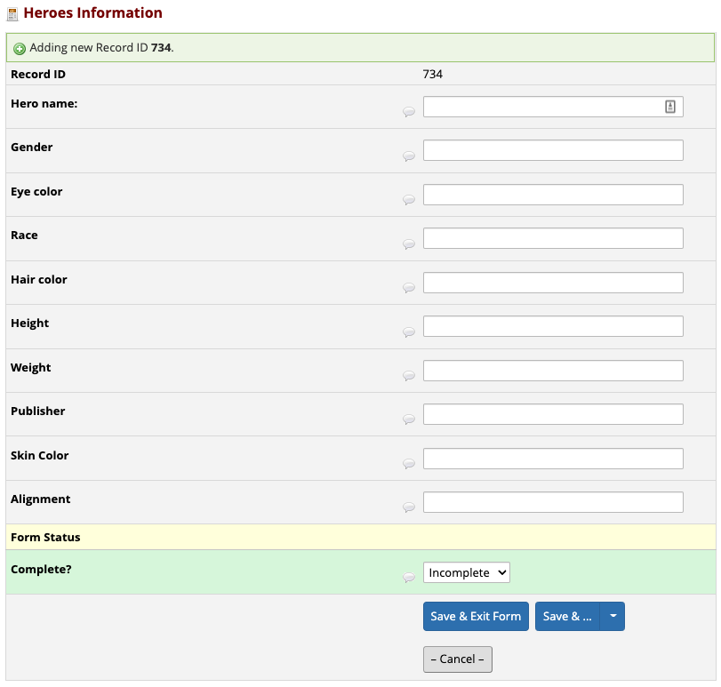
heroes_information instrumentNote that the label for name has a trailing colon
:. This won’t look good as a variable label so let’s remove
it. The make_labelled() function has a
format_labels argument that you can use to preprocess
labels before applying them to variables.
superheroes |>
  make_labelled(format_labels = ~ gsub(":", "", .)) |>
  bind_tibbles()

labelled::look_for(heroes_information, "hero")
#>  pos variable label     col_type missing values
#>  2   name     Hero name chr      0
Removing trailing : characters from a field label is a
fairly common operation, so REDCapTidieR provides a format helper function that you
can pass to the format_labels argument:
fmt_strip_trailing_colon("Hero name:")
#> [1] "Hero name"
To find out about other helpers included with REDCapTidieR, see
?`format-helpers`.
The format_labels argument will also accept multiple
functions in a vector or list. You can pass any function that takes a
character vector and returns a modified character vector to
format_labels. make_labelled() will process
the variable labels in the order that these functions are supplied. In
the following example, we remove the trailing colon with
fmt_strip_trailing_colon() and then make the labels lower
case with base::tolower().
superheroes |>
  make_labelled(
    format_labels = c(
      fmt_strip_trailing_colon,
      base::tolower
    )
  ) |>
  bind_tibbles()

labelled::look_for(heroes_information)
#>  pos variable             label                    col_type missing values
#>  1   record_id            record id                dbl      0
#>  2   name                 hero name                chr      0
#>  3   gender               gender                   chr      0
#>  4   eye_color            eye color                chr      0
#>  5   race                 race                     chr      0
#>  6   hair_color           hair color               chr      0
#>  7   height               height                   dbl      0
#>  8   weight               weight                   dbl      2
#>  9   publisher            publisher                chr      15
#>  10  skin_color           skin color               chr      0
#>  11  alignment            alignment                chr      0
#>  12  form_status_complete redcap instrument compl~ fct      0       Incomplete
#>                                                                     Unverified
#>                                                                     Complete
Adding summary statistics to the metadata with the skimr package
REDCapTidieR provides the add_skimr_metadata() function
to make it easy to compute summary statistics for fields of the project using the skimr package. The summary
statistics are added to metadata
tibbles. Below is a simple example showing some of the summaries
including count of missing values (n_missing), proportion
of non-missing values (complete_rate), and various numeric
statistics:
# Extract the heroes_information metadata tibble and add metadata
heroes_information_metadata <-
  superheroes |>
  add_skimr_metadata() |>
  dplyr::select(redcap_metadata) |>
  purrr::pluck(1, 1)

# Highlight the numeric summaries created by add_skimr_metadata()
heroes_information_metadata |>
  dplyr::select(field_name, skim_type:complete_rate, starts_with("numeric")) |>
  rmarkdown::paged_table()
This enables quick insights into data content and supports
exploratory data analytics. The columns added by
add_skimr_metadata() can also be labelled.
Package Options
REDCapTidieR allows you to set a couple options globally to avoid
passing extra arguments to read_redcap.
Globally allow mixed structure instruments:
options(redcaptidier.allow.mixed.structure = TRUE)Globally silence warnings related to Missing Data Codes (MDCs):
options(redcaptidier.allow.mdc = TRUE)As of v1.1.0, REDCapTidieR has partial support for MDCs. MDCs in
logical and categorical fields are converted to NA with a
warning. MDCs in all other field types remain in the output. If you need
greater support for MDCs, consider opening
an issue!