Diving Deeper: Understanding REDCapTidieR Data Tibbles
Source:vignettes/articles/diving_deeper.Rmd
diving_deeper.RmdThe Block Matrix
In the Getting Started vignette, we stated that importing records from complex REDCap projects via the REDCap API can be ugly. In this section we will describe what we mean by this in more precise language.
The REDCapR::redcap_read_oneshot() function pulls data
from a REDCap project via the REDCap
API and provides it to the R environment without performing much
processing. It returns a list with an element named data
that contains all of the data of the project as a single data frame.
Below, we use this function to import data from the Superhero
REDCap database, which contains a nonrepeating
instrument heroes_information and a repeating
instrument super_hero_powers. We use
rmarkdown::paged_table() to allow you to explore this large
data frame in the browser.
superheroes_token <- "123456789ABCDEF123456789ABCDEF04"
redcap_uri <- "https://my.institution.edu/redcap/api/"
superheroes_ugly <- REDCapR::redcap_read_oneshot(redcap_uri, superheroes_token)$data

superheroes_ugly |>
  rmarkdown::paged_table()
This data structure is called a block matrix. It’s what happens when REDCap mashes the contents of a project that has both repeating and nonrepeating instruments into a single table.
While it may seem a good idea to have everything in one data frame, there are significant downsides, including:
It’s unwieldy! Although there are only 734 superheroes in the data set, there are 6,700 rows. Every transformation first requires whittling down a huge data set.
There are a lot of
NAvalues. Many of theseNAvalues don’t represent fields left blank during data entry but instead are an artifact of how the table is generated.Metadata that would be helpful is missing. For example, it’s not possible to determine which columns are associated with a specific instrument for nonrepeating instruments.
The meaning of a row in the data set is inconsistent. Some rows represent observations on a per-record level (i.e. those derived from nonrepeating instruments) and others represent observations on a per-repeat-instance level (i.e. those derived from repeating instruments). This technically violates the definition of Tidy Data because multiple types of observational units are stored in the same table.
Structure of REDCapTidieR Data Tibbles
REDCapTidieR breaks the block matrix up into data tibbles, one for each instrument. REDCapTidieR then collects the data tibbles as a list column in a special object we call the supertibble.
These data tibbles are tidier than the block matrix because one instrument can only be repeating or nonrepeating, and therefore each data tibble can only have one type of observational unit stored inside of it. Each data tibble has consistent granularity.
Let’s take a look at the data tibbles derived from the Superhero
database and contrast them with the block matrix. Consider
heroes_information, which contains data from a
nonrepeating instrument. This tibble is much smaller
than the block matrix at 734 rows by 12 columns, and there are no
NAs. The data tibble’s name heroes_information
is descriptive. REDCapTidieR knows the names of all instruments because
in addition to querying the project’s data it also queries the project’s
metadata which describes, among other things, the names of REDCap
instruments. Each entry has the same granularity, one
superhero, identified by its record_id. A
number of data columns follow,
starting with name, gender,
eye_color, race, etc. These columns are in the
same order as on the REDCap instrument. The last column of a
REDCapTidieR data tibble is always form_status_complete
which indicates whether the instrument has been marked as completed.
library(REDCapTidieR)

read_redcap(redcap_uri, superheroes_token) |>
  bind_tibbles()

heroes_information |>
  rmarkdown::paged_table()
Now consider the super_hero_powers table, which contains
data from a repeating instrument. In addition to
record_id there is a redcap_form_instance
column. The granularity of each row is one superpower per
superhero, identified by its record_id and
redcap_form_instance. Because these two columns uniquely
identify a row in the data tibble, we call them identifier
columns. In the REDCapTidieR supertibble, identifier
columns always come first, followed by [data columns]
and finally the form_status_complete column.
super_hero_powers |>
  rmarkdown::paged_table()
Longitudinal REDCap Projects
REDCap supports two main mechanisms to allow collecting the same data multiple times: repeating instruments and longitudinal projects. In addition, a longitudinal project may have arms and/or repeating events.
The granularity of each table (i.e. the observational unit that a single row represents) depends on the structure of the project (classic, longitudinal, longitudinal with multiple arms), the structure of the instrument (repeating or nonrepeating), and, for longitudinal projects, the structure of the event (repeating or nonrepeating). Note that REDCap does not support repeating instruments inside a repeating event. REDCapTidieR generates identifier columns according to the following table:
| Instrument Structure | Event Structure | Classic | Longitudinal, one arm | Longitudinal, multi-arm |
|---|---|---|---|---|
| Nonrepeating | Nonrepeating | record_id |
record_id +redcap_event
|
record_id +redcap_event +redcap_arm
|
| Repeating | Nonrepeating |
record_id +redcap_form_instance
|
record_id +redcap_form_instance +redcap_event
|
record_id +redcap_form_instance +redcap_event +redcap_arm
|
| Nonrepeating | Repeating | N/A |
record_id +redcap_event_instance +redcap_event
|
record_id +redcap_event_instance +redcap_event +redcap_arm
|
| Repeating | Repeating | Not Supported | Not Supported | Not Supported |
Note: Taken in combination, the identifier columns of any REDCapTidieR tibble are guaranteed to be unique and can therefore be used as composite primary key. This makes it easy to join REDCapTidieR tibbles to one another!
By default, REDCap names the record ID field record_id,
but this can be changed inside the REDCap project, and REDCapTidieR is
smart enough to handle this. For example, if the record ID field was
renamed to subject_id then the record ID column of each
data tibble would be subject_id. Whatever its name, the
record ID column is always the first identifier column and is always the
first column of a REDCapTidieR data tibble. Additional columns are
generated in the order shown in the table above.
Let’s look at a REDCap database you might use to capture data for a
clinical trial. This is a longitudinal database that assesses some data
(e.g. demographics) just once at enrollment, and other data
(e.g. physical exam or labs) multiple times at pre-defined study visits.
We use dplyr::select() here to highlight instrument names
and whether or not each instrument is repeating. This database has six
nonrepeating and three repeating instruments.
longitudinal_token <- "123456789ABCDEF123456789ABCDEF06"
library(REDCapTidieR)

longitudinal <- read_redcap(redcap_uri, longitudinal_token)

longitudinal |>
  dplyr::select(redcap_form_name, redcap_form_label, structure) |>
  rmarkdown::paged_table()
The demographics instrument is nonrepeating. The
granularity is one row per study subject per event, but since it is only designated
for a single event, it is really one row per study subject. The
redcap_event column identifies the name of the event with
which the instrument is associated: screening__enrollm
(Screening and Enrollment).
longitudinal |>
  bind_tibbles()

demographics |>
  rmarkdown::paged_table()
The chemistry instrument is nonrepeating as well.
However, it is designated for multiple events because chemistry labs are
drawn at multiple study visits. The redcap_event column
shows that we have chemistry data from four different
events. The granularity is one row per study subject per event. Each of
the three subjects has multiple rows. Each row is identified by the
combination of subject_id and
redcap_event.
chemistry |>
  rmarkdown::paged_table()
The adverse_events instrument is
repeating. Since adverse events aren’t tied to specific
study visits, and a patient can have any number of different adverse
events at any time, it makes sense to designate this instrument to a
single special event adverse_event, which is what we’ve
done here. The granularity of this table is one row per study subject
per repeat instance per event. However since it is only designated for a
single event, it is really one row per study subject per repeat
instance. The first subject has three adverse events listed, and the
second subject has two.
adverse_events |>
  rmarkdown::paged_table()
It is possible to have a repeating instrument designated to multiple events, however this is an uncommon pattern. REDCapTidieR supports this scenario as well.
The unscheduled event is a
repeating event. Like adverse events, unscheduled
visits aren’t tied to a pre-determined study visit, and a patient could
have zero, one, or multiple unscheduled visits. On the other hand, you
might want to record the same kinds of data for an unscheduled visit as
for a pre-determined regular visit and collect data in the same
instruments, for example physical_exam and
hematology. The granularity of these tables is one row per
study subject per event per event instance. The subject had two
unscheduled visits. redcap_event_instance allows us to
match physical_exam and hematology responses
which occurred on the same unscheduled visit.
physical_exam |>
  dplyr::filter(redcap_event == "unscheduled") |>
  rmarkdown::paged_table()

hematology |>
  dplyr::filter(redcap_event == "unscheduled") |>
  rmarkdown::paged_table()
Note that REDCapTidieR allows for an instrument to be associated with
both repeating and nonrepeating events at the same time. In this case,
the the redcap_event_instance column will be
NA in rows that correspond with data captured as part of a
nonrepeating event.
REDCapTidieR supports projects with multiple arms. If you have a
project with multiple arms, there will be an additional column
redcap_arm to identify the arm that the row is associated
with.
Mixed Structure Instruments
By default, REDCapTidieR does not allow you to have the same instrument designated both as a repeating and as a nonrepeating instrument in different events (i.e. a “mixed structure instrument”), and will throw an error if this is detected:
Error in `clean_redcap_long()` at REDCapTidieR/R/read_redcap.R:272:5:
✖ Instruments detected that have both repeating and nonrepeating instances defined in the project: mixed_structure_1 and mixed_structure_form_complete
ℹ Set `allow_mixed_structure` to `TRUE` to override. See Mixed Structure Instruments for more information.
This is because such a design inherently goes against tidy data principles.
However, as of REDCapTidieR v1.1.0 it is now possible to override
this behavior by setting allow_mixed_structure in
read_redcap() to TRUE. When enabled,
nonrepeating variants of mixed structure instruments will be treated as
repeating instruments with a single repeating instance.
Users are cautioned when enabling this feature, since it changes
definitions in the original data output. To visually assist with this,
you will see that structure in the supertibble will say “mixed”:
read_redcap(redcap_uri,
  mixed_token,
  allow_mixed_structure = TRUE
) |>
  rmarkdown::paged_table()
Categorical Variables
REDCapTidieR performs a number of opinionated transformations on categorical fields to streamline exploring them and working with them.
Fields that are of type
yesno or truefalse are converted to
logical variables.
adverse_events$adverse_event_serious |>
  dplyr::glimpse()
#>  logi [1:5] FALSE FALSE FALSE FALSE FALSE
Fields of single-answer categorical type (dropdown,
radio) are converted to factor variables by
default. REDCapTidieR constructs this factor in such a way that the all
possible choices defined in REDCap
are represented as factor levels, and that the order of the factor
levels is the same as the order of choices in REDCap.
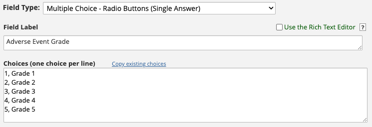
Consider the Field Editor for the adverse_event_grade
variable which is a single-answer radio field. There are
five choices for this field. Choices have raw values
and choice labels, separated by a comma. Here, the raw
values are 1, 2, 3,
4, and 5, and their associated choice labels
are Grade 1, Grade 2, Grade 3,
Grade 4, and Grade 5.
REDCapTidieR preserves all the possible choices as levels even if not all of them are represented in the data. This makes it possible to discover all of the different choices. For example, even though we have only Grade 1 and 2 adverse events in the data, we can see that there are 5 possible grades.
adverse_events$adverse_event_grade
#> [1] Grade 2 Grade 1 Grade 1 Grade 2 Grade 1
#> Levels: Grade 1 Grade 2 Grade 3 Grade 4 Grade 5
Adverse event grades are intrinsically ordered. When a multiple choice field has intrinsically ordered choices, those choices are usually presented in the proper order. Since REDCapTidieR preserves the order of choices from REDCap, you can convert intrinsically ordered variables to ordered factors.
ae_grade <- adverse_events$adverse_event_grade

ae_grade |>
  factor(ordered = TRUE, levels = levels(ae_grade))
#> [1] Grade 2 Grade 1 Grade 1 Grade 2 Grade 1
#> Levels: Grade 1 < Grade 2 < Grade 3 < Grade 4 < Grade 5
Fields of the multi-answer checkbox type are treated in
a special way. REDCapTidieR expands these fields into multiple
columns. Each of these derived columns represents one
choice and is coded as a logical
variable.
Consider the adverse_event_relationship_other field.
This field has eight choices, and their raw values (i.e. the part before
the comma) are apheresis, ld_chemo,
soc_treatment, underlying_disease,
other_research_proc, con_meds, and
other.
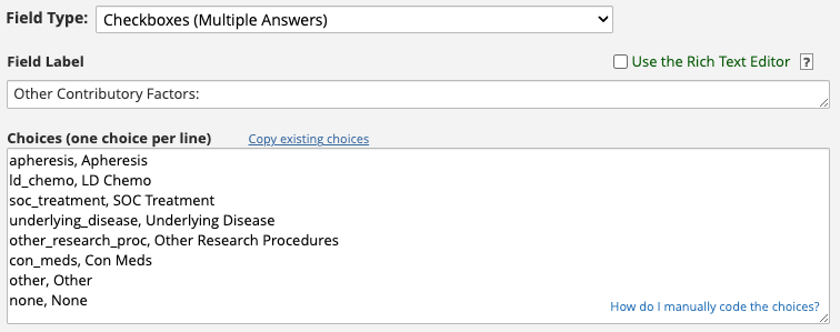
We recommend that for multi-answer
checkboxfields you make the raw value a human readable word as we do in the above example.
REDCapTidieR will construct the name of each variable from the name
of the field, followed by three underscores, followed by the
raw value of the choice defined in REDCap. Here are the
variables REDCapTidieR generates from the
adverse_event_relationship_other field:
adverse_events |>
  dplyr::select(dplyr::starts_with("adverse_event_relationship_other___")) |>
  dplyr::glimpse()
#> Rows: 5
#> Columns: 8
#> $ adverse_event_relationship_other___apheresis           <lgl> FALSE, FALSE, F…
#> $ adverse_event_relationship_other___ld_chemo            <lgl> FALSE, FALSE, F…
#> $ adverse_event_relationship_other___soc_treatment       <lgl> FALSE, FALSE, F…
#> $ adverse_event_relationship_other___underlying_disease  <lgl> TRUE, FALSE, FA…
#> $ adverse_event_relationship_other___other_research_proc <lgl> FALSE, FALSE, F…
#> $ adverse_event_relationship_other___con_meds            <lgl> TRUE, FALSE, TR…
#> $ adverse_event_relationship_other___other               <lgl> FALSE, FALSE, F…
#> $ adverse_event_relationship_other___none                <lgl> FALSE, TRUE, FA…
Parsed Data Type Validation
REDCap returns export data in a format where column types must be inferred. In sparse projects (for example, columns with many missing values), automatic parsing may occasionally infer an unexpected R type for a field.
read_redcap() checks parsed column types against REDCap
metadata and warns if there is a likely mismatch. This warning is
intended to flag cases where a field may have been parsed in a way that
could affect downstream analysis.
| REDCap field type | Allowed R type | Notes |
|---|---|---|
text, notes, calc,
dropdown, radio
|
character, double, integer,
factor, date, time,
datetime
|
When parsed as logical, warns only when
non-NA value is present. |
file |
character |
When parsed as logical, warns only when
non-NA value is present. |
slider |
double, integer
|
When parsed as logical, warns only when
non-NA value is present. |
checkbox, yesno,
truefalse
|
character, logical, double,
integer
|
When this occurs, use col_types to explicitly enforce
expected parsing behavior:
read_redcap(
  redcap_uri,
  superheroes_token,
  col_types = readr::cols(
    weight = readr::col_integer()
  )
) |>
  extract_tibble("heroes_information") |>
  rmarkdown::paged_table()
Data Access Groups
Some REDCap projects may use Data Access Groups (DAGs) to assign specific user privileges and record-level access to entries within the project. DAGs are frequently used in multi-center projects where the data from an individual centers needs to be isolated and protected from users belonging to other centers.
If a project has DAGs
enabled, by default a column named redcap_data_access_group
will appear in each data tibble
after the identifier
columns.
redcap_project_with_dags <- read_redcap(redcap_uri, dag_token)

redcap_project_with_dags |>
  extract_tibble("non_repeat_form_1") |>
  rmarkdown::paged_table()
Surveys
Instruments that are used to generate REDCap surveys generate additional data columns:
redcap_survey_timestamp: the time at which the survey was competedredcap_survey_identifier: the participant identifier. This will beNAif the Participant Identifier feature in REDCap is disabled.
These columns are placed after all of the other data columns and
prior to the form_status_complete column.
survey <- read_redcap(redcap_uri, survey_token) |>
  extract_tibble("survey")

survey |>
  dplyr::glimpse()
#> Rows: 4
#> Columns: 9
#> $ record_id                <dbl> 1, 2, 3, 4
#> $ survey_yesno             <lgl> TRUE, FALSE, NA, NA
#> $ survey_radio             <fct> Choice 1, Choice 2, NA, NA
#> $ survey_checkbox___one    <lgl> FALSE, FALSE, FALSE, FALSE
#> $ survey_checkbox___two    <lgl> TRUE, TRUE, FALSE, FALSE
#> $ survey_checkbox___three  <lgl> TRUE, TRUE, FALSE, FALSE
#> $ redcap_survey_identifier <lgl> NA, NA, NA, NA
#> $ redcap_survey_timestamp  <dttm> 2022-11-09 10:33:35, NA, NA, NA
#> $ form_status_complete     <fct> Complete, Incomplete, Incomplete, Incomplete
Summary
In summary, here are the rules by which REDCapTidieR constructs data tibbles:
- One data tibble is built for each instrument.
- The first column is always the record ID column which is derived from the record ID field.
- Additional identifier columns may follow the record ID column, depending on the structure of the instrument and the structure of the project (see the table above).
- If the project has data access groups enabled, a column identifying the data access column will follow here.
- Next, data columns appear in the same order as in the REDCap instrument. True/false type fields are converted to logical columns. Single-answer categorical fields are converted to factor columns. Multi-answer checkbox fields are expanded to a set of logical columns, one for each choice.
- If the instrument is used as a survey, the survey timestamp and identifier columns will appear next.
- The final column is always
form_status_complete.