Adding arrows to ggswim

It can be useful to visually indicate the continuation of specific records in a swimmer plot. Adding arrows to the tail ends of swimmer plot lanes in ggswim can help communicate subject survival status, such as whether or not a subject is still on a given study. Use this article when the README example is not enough and you need more control over arrow placement, styling, or legends.

To facilitate the addition of arrows, we provide geom_swim_arrow() as a way to attach continuation indicators to swimmer plot lanes. Behind the scenes, arrows are drawn with ggplot2::geom_segment(). When only xend is mapped, geom_swim_arrow() treats xend as the lane endpoint and extends a fixed-length arrow neck to the right. When both x and xend are mapped, the arrow extent is data-driven. geom_swim_arrow() gives users control over arrow neck and head length, along with options for colour/color, fill, and type; refer to ?geom_swim_arrow for detailed information.

Arrow appearance can be specified in two ways:

• directly via parameters such as arrow_colour, arrow_fill, and arrow_type
• by mapping the arrow aesthetic and supplying styles through scale_arrow_discrete()

geom_swim_arrow() does not replace the ability to use the arrow parameter in geom_swim_lane(). As mentioned, geom_swim_lane() comes with nearly all of the same capabilities as geom_segment(), but it may be more challenging to apply arrows as expected depending on how your data is structured.

Adding arrows using geom_swim_arrow()

To demonstrate how you might add arrows onto the patient_data dataset, let’s take a subset of patient_data that would help us make use of geom_swim_arrow():

library(ggswim)
library(ggplot2)

arrow_data <- patient_data |>
  dplyr::left_join(
    end_study_events |>
      dplyr::select(pt_id, label),
    by = "pt_id"
  ) |>
  dplyr::select(pt_id, end_time, label) |>
  dplyr::filter(.by = pt_id, end_time == max(end_time)) |>
  dplyr::filter(is.na(label)) |>
  unique()

arrow_data
#> # A tibble: 8 × 3
#>   pt_id end_time label
#>   <chr>    <dbl> <chr>
#> 1 04         9   NA   
#> 2 09        12   NA   
#> 3 13         2.5 NA   
#> 4 14         0.9 NA   
#> 5 15         0.9 NA   
#> 6 17         2.8 NA   
#> 7 18         3.3 NA   
#> 8 19         6   NA

This dataset is derived from patient_data joined to end-study labels. Since populated labels in end_study_events mean a subject went off study, arrows are only applicable for subjects with no end-study status. Now let’s use geom_swim_arrow() in combination with geom_swim_lane() to make a swimmer plot:

patient_data |>
  ggplot() +
  geom_swim_lane(
    mapping = aes(
      x = start_time, xend = end_time, y = pt_id,
      color = disease_assessment
    ),
    linewidth = 5
  ) +
  geom_swim_arrow(
    data = arrow_data,
    mapping = aes(xend = end_time, y = pt_id),
    arrow_neck_length = 5,
    arrow_head_length = grid::unit(0.15, "inches"),
    arrow_colour = "firebrick",
    arrow_fill = "gold"
  )

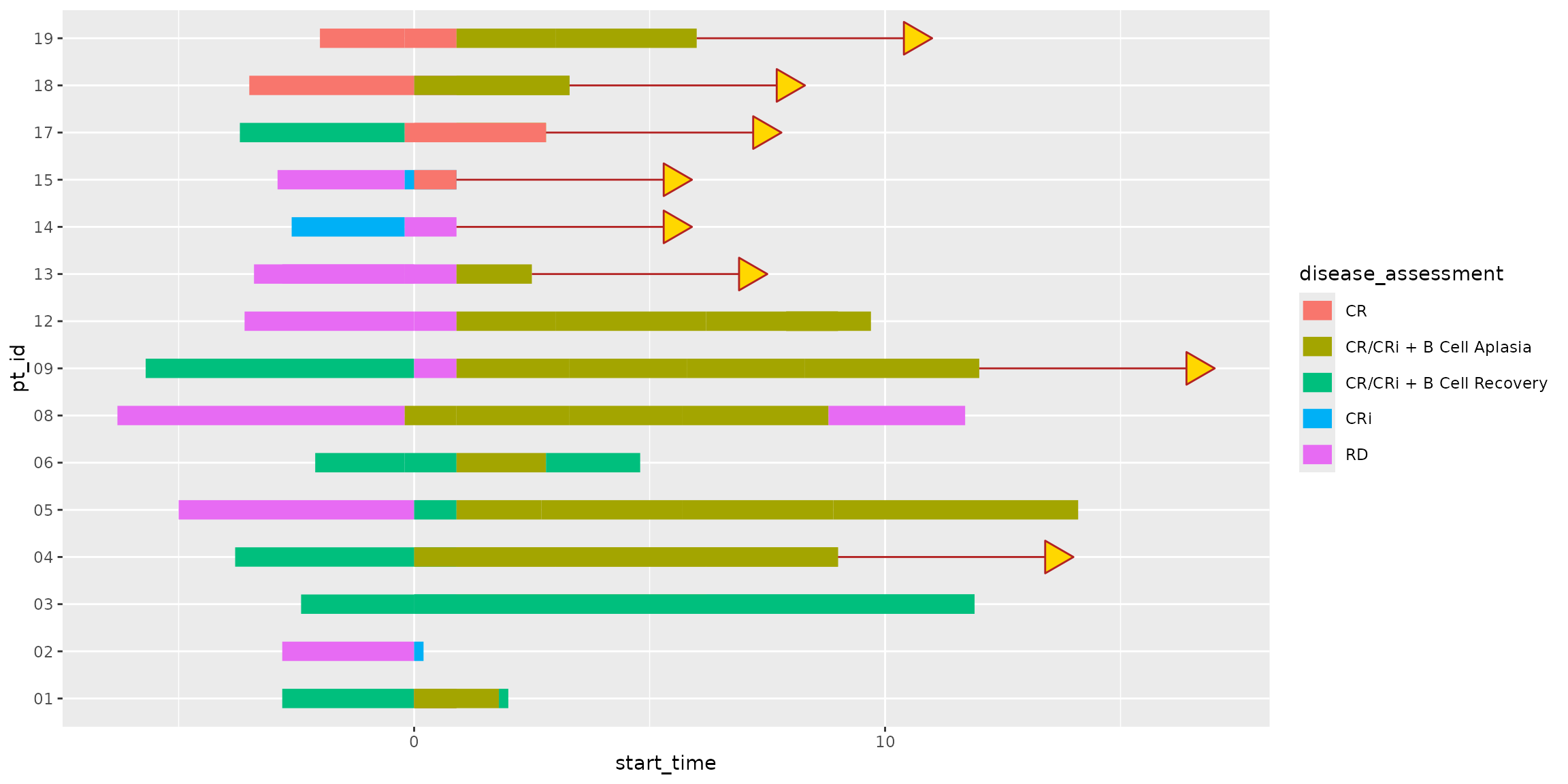
Here we’ve assigned arrows to only the subset of patients that have not met an end-of-study event. Note that geom_swim_arrow() gives control over the arrow head, neck, colour/color, shape, and length.

geom_swim_arrow() also allows aesthetically mapped x start and xend values. If you would prefer arrow neck lengths to come from your data, supply both x and xend in aes().

Using scale_arrow_discrete() for arrow styling

In addition to specifying arrow appearance directly through parameters, arrows can also be styled using the arrow aesthetic together with scale_arrow_discrete(). This approach allows arrow styles to be controlled through the ggplot2 scaling system, making it easier to add arrows as their own legend component or to manage multiple arrow styles.

To demonstrate this approach, we can map a value to the arrow aesthetic and then define its appearance using scale_arrow_discrete():

patient_data |>
  ggplot() +
  geom_swim_lane(
    mapping = aes(
      x = start_time, xend = end_time, y = pt_id,
      color = disease_assessment
    ),
    linewidth = 5
  ) +
  geom_swim_arrow(
    data = arrow_data,
    mapping = aes(
      xend = end_time,
      y = pt_id,
      arrow = "Continuation"
    ),
    arrow_neck_length = 5,
    arrow_head_length = grid::unit(0.15, "inches")
  ) +
  scale_arrow_discrete(
    limits = "Continuation",
    colours = "firebrick",
    fills = "gold",
    types = "closed",
    name = NULL
  )

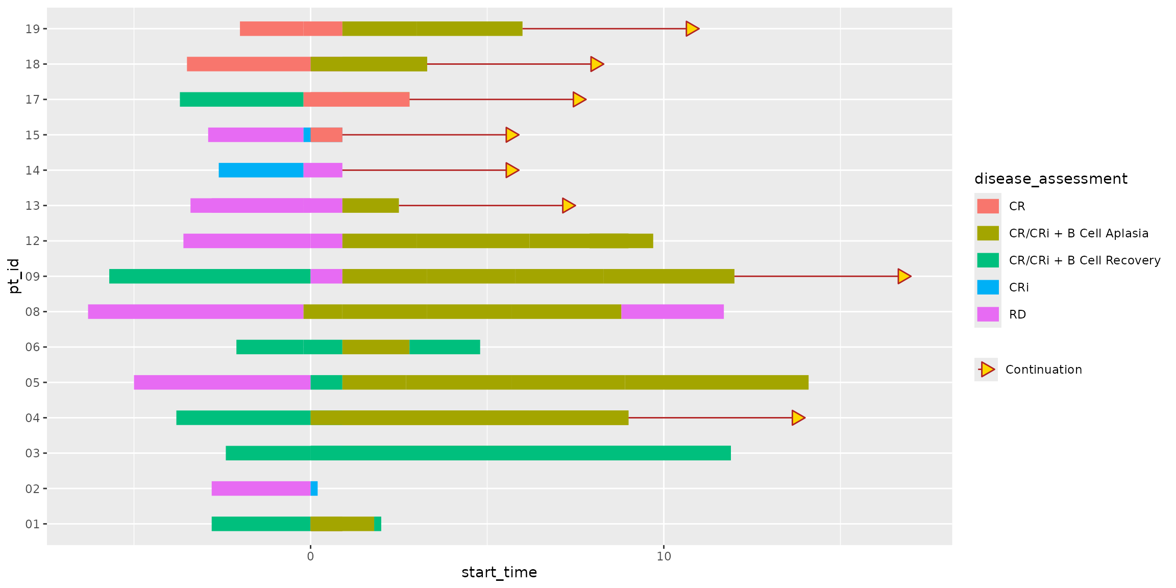
Here, the “Continuation” value mapped to the arrow aesthetic is used by scale_arrow_discrete() to determine the arrow’s visual properties. Because this mapping is treated like any other discrete scale in ggplot2, it can also be displayed as a separate legend entry if desired.

Using scale_arrow_discrete() is particularly helpful when:

• arrows should appear as a dedicated legend component
• multiple arrow styles are required
• arrow styling should be managed consistently across plots

For simple cases, specifying arrow parameters directly in geom_swim_arrow() may still be sufficient. However, using scale_arrow_discrete() provides a more flexible and scalable approach when working with more complex swimmer plots.