Gallery

library(ggswim)
library(ggplot2)
library(dplyr)

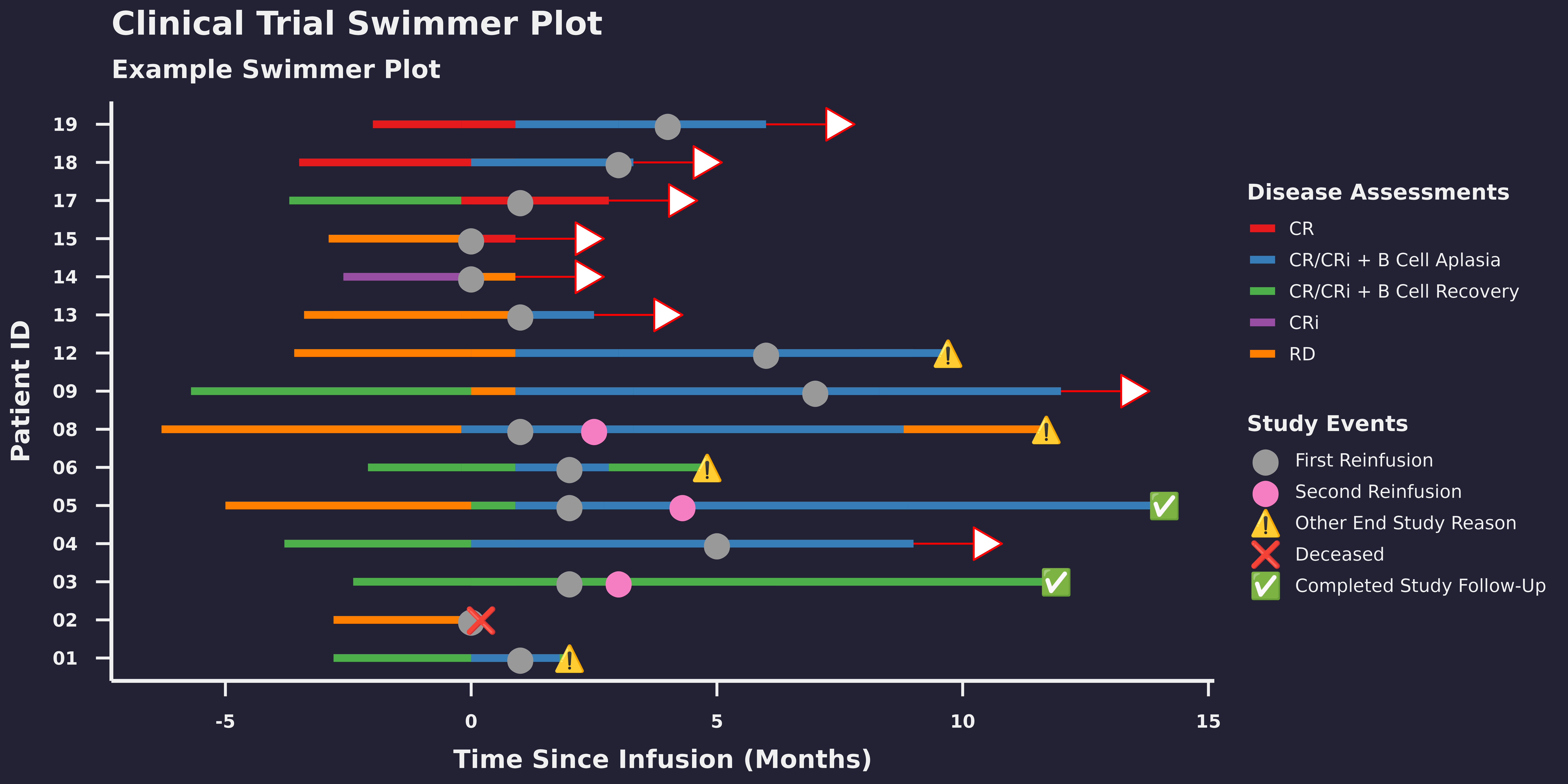
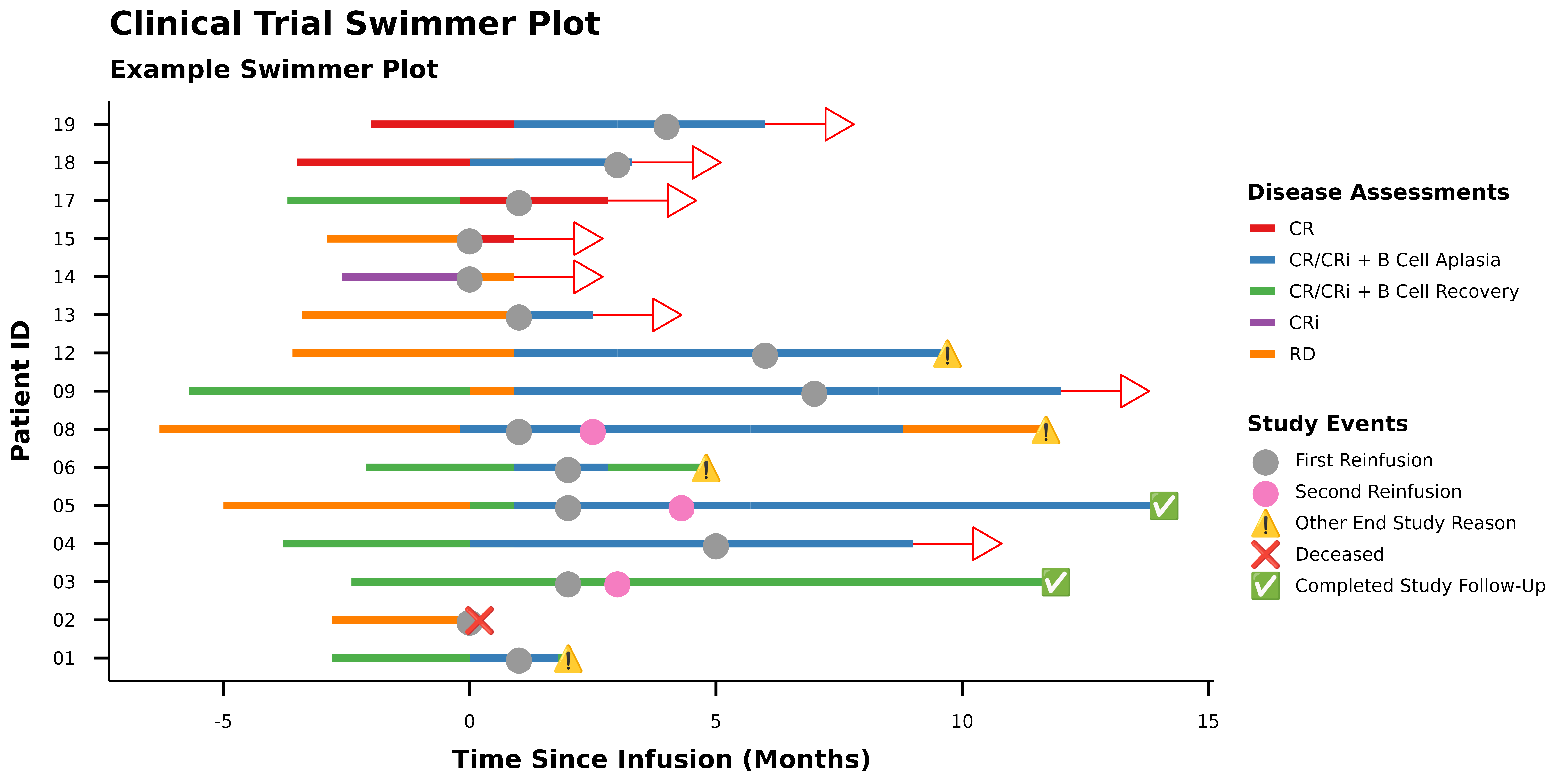
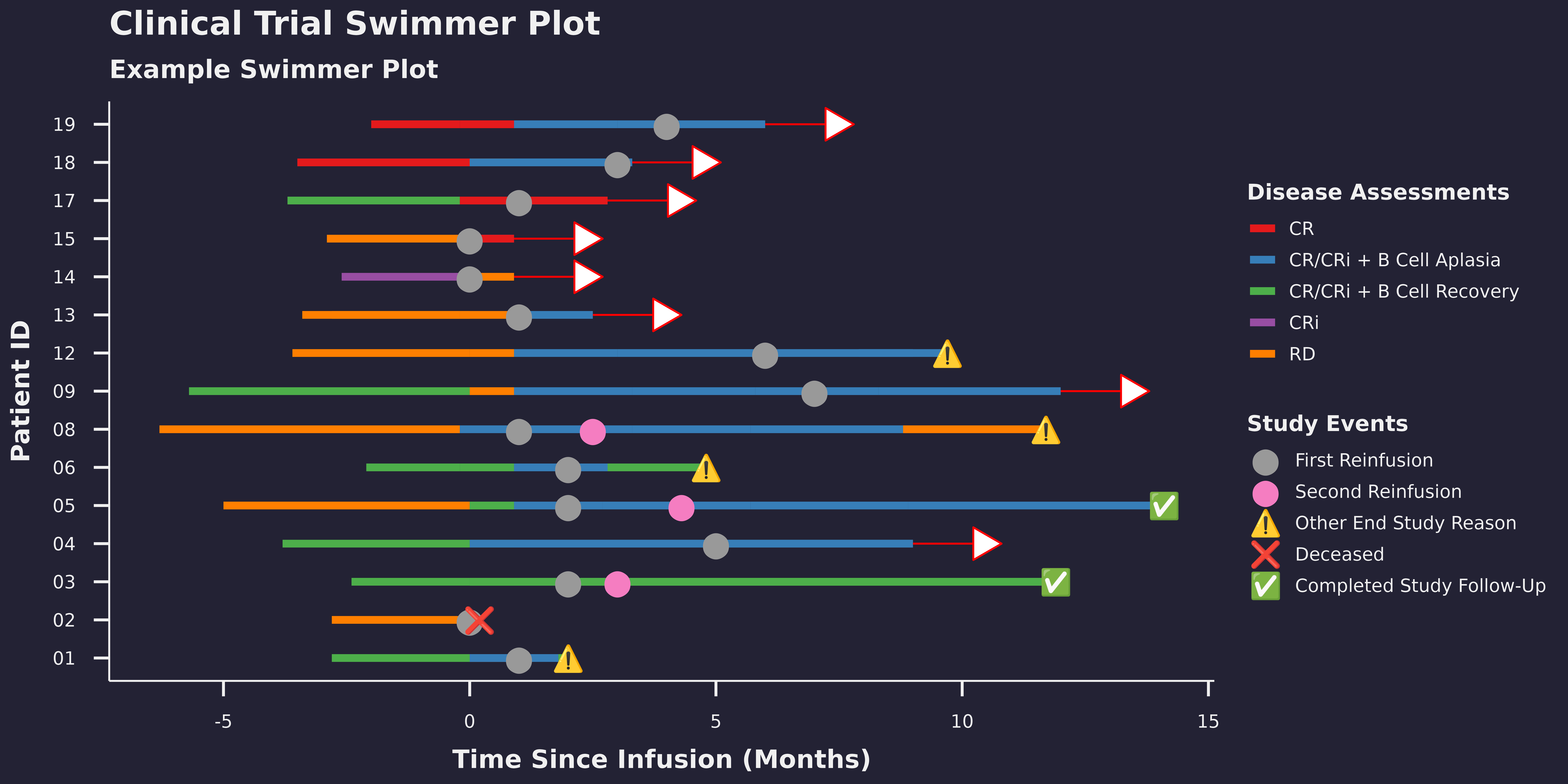
Random Data Sets

In this example, we’ll set up some random data for reproducibility by defining dataframes for our lanes and our markers.

set.seed(123)
lane_data <- tibble(
  x = 0,
  xend = sample(5:20, 30, replace = TRUE),
  y = factor(rep(1:15, each = 2)),
  colour = sample(c("red", "blue", "green", "yellow", "purple"), 30, replace = TRUE)
)

set.seed(123)
marker_data <- tibble(
  x = sample(5:20, 30, replace = TRUE),
  y = factor(rep(1:15, each = 2)),
  label = sample(c("A", "B", "C", "D", "E"), 30, replace = TRUE),
  glyph = NA
) |>
  mutate(
    glyph = dplyr::case_when(
      label == "A" ~ "😊",
      label == "B" ~ "🎉",
      label == "C" ~ "✅",
      label == "D" ~ "💥",
      label == "E" ~ "✨",
      .default = NA
    )
  )

And then we’ll call those dataframes into their appropriate swim and marker geom functions:

ggplot() +
  geom_swim_lane(
    data = lane_data,
    aes(x = x, xend = xend, y = y, colour = colour),
    linewidth = 3
  ) +
  geom_swim_marker(
    data = marker_data,
    aes(x = x, y = y, marker = label),
    size = 8
  ) +
  scale_colour_brewer(name = "Lanes", palette = "Set1") +
  with(
    marker_data,
    scale_marker_discrete(glyphs = glyph, limits = label, name = "Markers")
  ) +
  labs(
    title = "Sample Swimmer Plot",
    x = "Time", y = "Record ID"
  ) +
  theme_ggswim()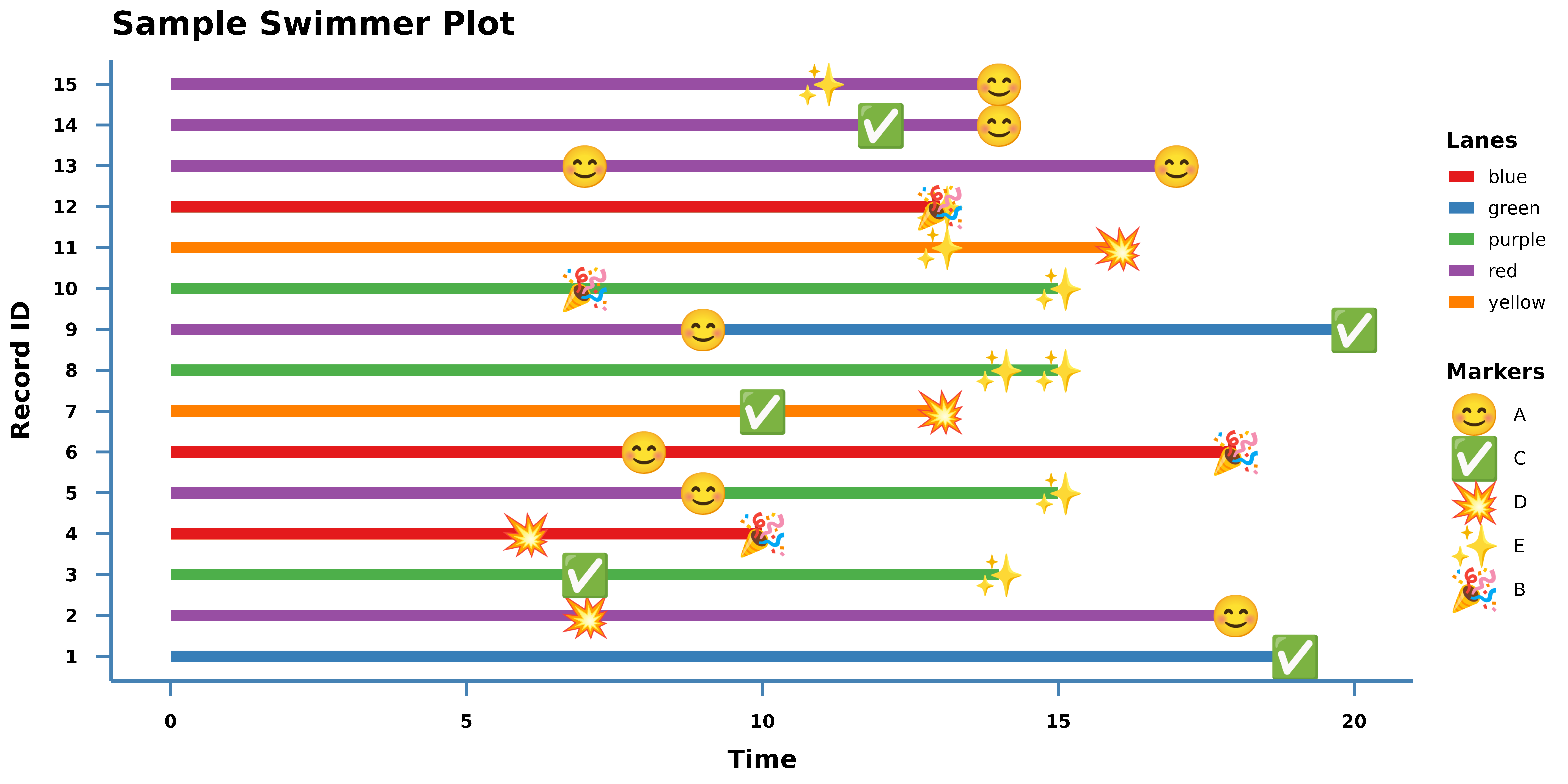

Using FontAwesome Icons

Next, we’ll replace the emojis above with calls to fontawesome() icons after first loading fonts with load_fonts():

# Load fonts from the ggswim GitHub repository
load_fonts(verbose = FALSE)

marker_data <- marker_data |>
  mutate(
    glyph = dplyr::case_when(
      label == "A" ~ fontawesome("fa-car"),
      label == "B" ~ fontawesome("fa-check"),
      label == "C" ~ fontawesome("fa-user"),
      label == "D" ~ fontawesome("fa-cat"),
      label == "E" ~ fontawesome("fa-dog"),
      .default = NA
    )
  )

ggplot() +
  geom_swim_lane(
    data = lane_data,
    aes(x = x, xend = xend, y = y, colour = colour),
    linewidth = 3
  ) +
  geom_swim_marker(
    data = marker_data,
    aes(x = x, y = y, marker = label),
    size = 8, family = "FontAwesome-Solid"
  ) +
  scale_colour_brewer(name = "Lanes", palette = "Set1") +
  with(
    marker_data,
    scale_marker_discrete(glyphs = glyph, limits = label, name = "Markers")
  ) +
  labs(
    title = "Sample Swimmer Plot",
    x = "Time", y = "Record ID"
  ) +
  theme_ggswim()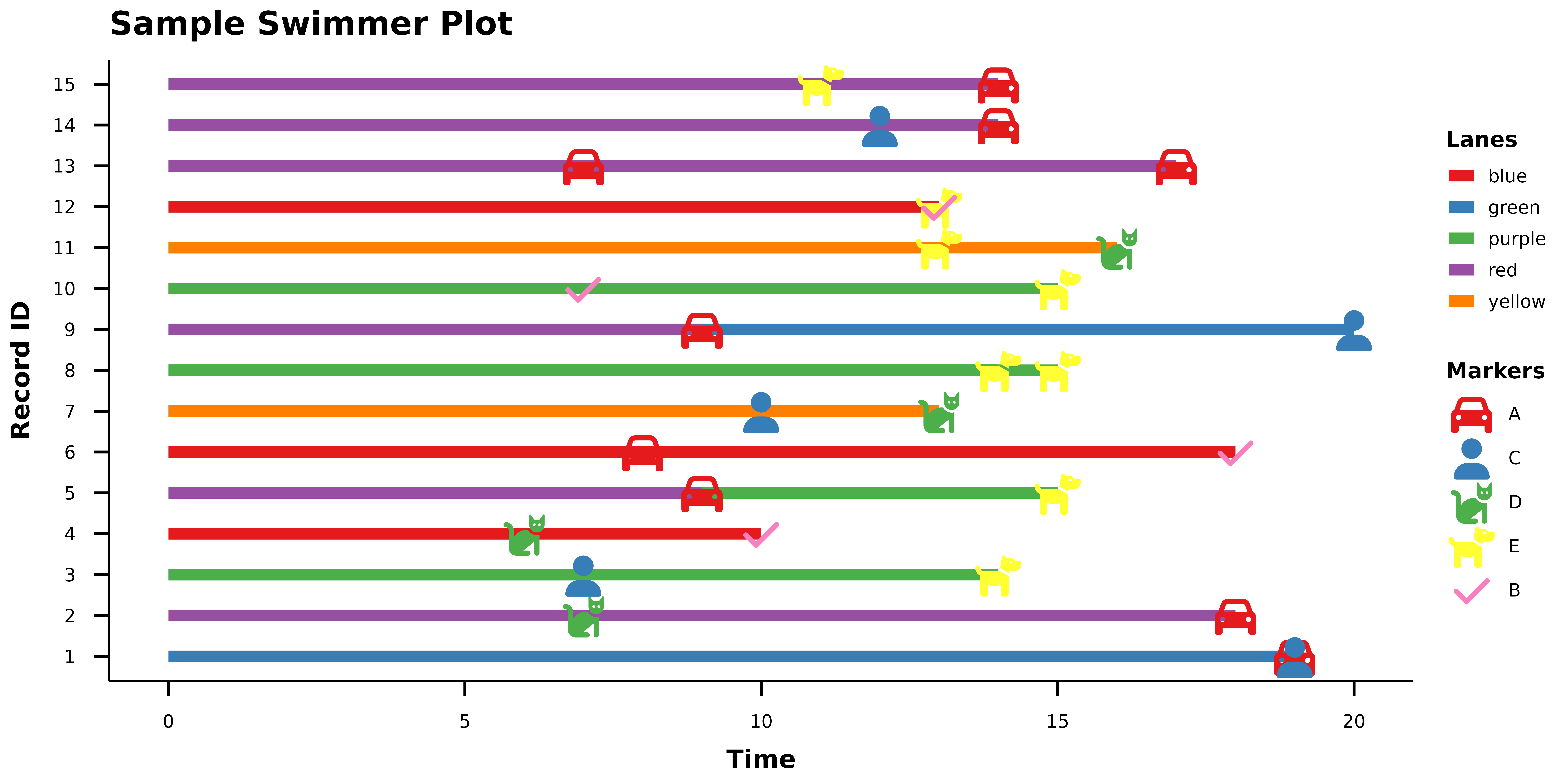

Be sure to specify the appropriate family argument in geom_swim_marker(). For FontAwesome the following are available:

• “FontAwesome-Solid”
• “FontAwesome-Regular”
• “FontAwesome-Brands”

You can use search_fontawesome() to check what icons are available to use.

ggswim supports FontAwesome free icons through the open source license.

Using Bootstrap Icons

We can similarly use Bootstrap icons with bootstrap():

marker_data <- marker_data |>
  mutate(
    glyph = dplyr::case_when(
      label == "A" ~ bootstrap("bs-car-front"),
      label == "B" ~ bootstrap("bs-folder-fill"),
      label == "C" ~ bootstrap("bs-clock-fill"),
      label == "D" ~ bootstrap("bs-check-circle-fill"),
      label == "E" ~ bootstrap("bs-chat-fill"),
      .default = NA
    )
  )

ggplot() +
  geom_swim_lane(
    data = lane_data,
    aes(x = x, xend = xend, y = y, colour = colour),
    linewidth = 3
  ) +
  geom_swim_marker(
    data = marker_data,
    aes(x = x, y = y, marker = label),
    size = 8, family = "Bootstrap"
  ) +
  scale_colour_brewer(name = "Lanes", palette = "Set1") +
  with(
    marker_data,
    scale_marker_discrete(glyphs = glyph, limits = label, name = "Markers")
  ) +
  labs(
    title = "Sample Swimmer Plot",
    x = "Time", y = "Record ID"
  ) +
  theme_ggswim()

Be sure to specify the appropriate family argument in geom_swim_marker(). For Bootstrap you only need to specify “Bootstrap”.

You can use search_bootstrap() to check what icons are available to use.

ggswim supports Bootstrap free icons through the open source license.

Themeing with ggswim

Here we’ll demonstrate some of the theme functions available with ggswim. These examples will use the same plot setup from the README, starting with the original output:

p

theme_ggswim()

p + theme_ggswim()

theme_ggswim_dark()

p + theme_ggswim_dark()